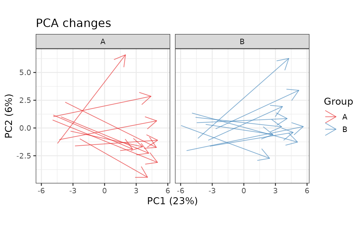
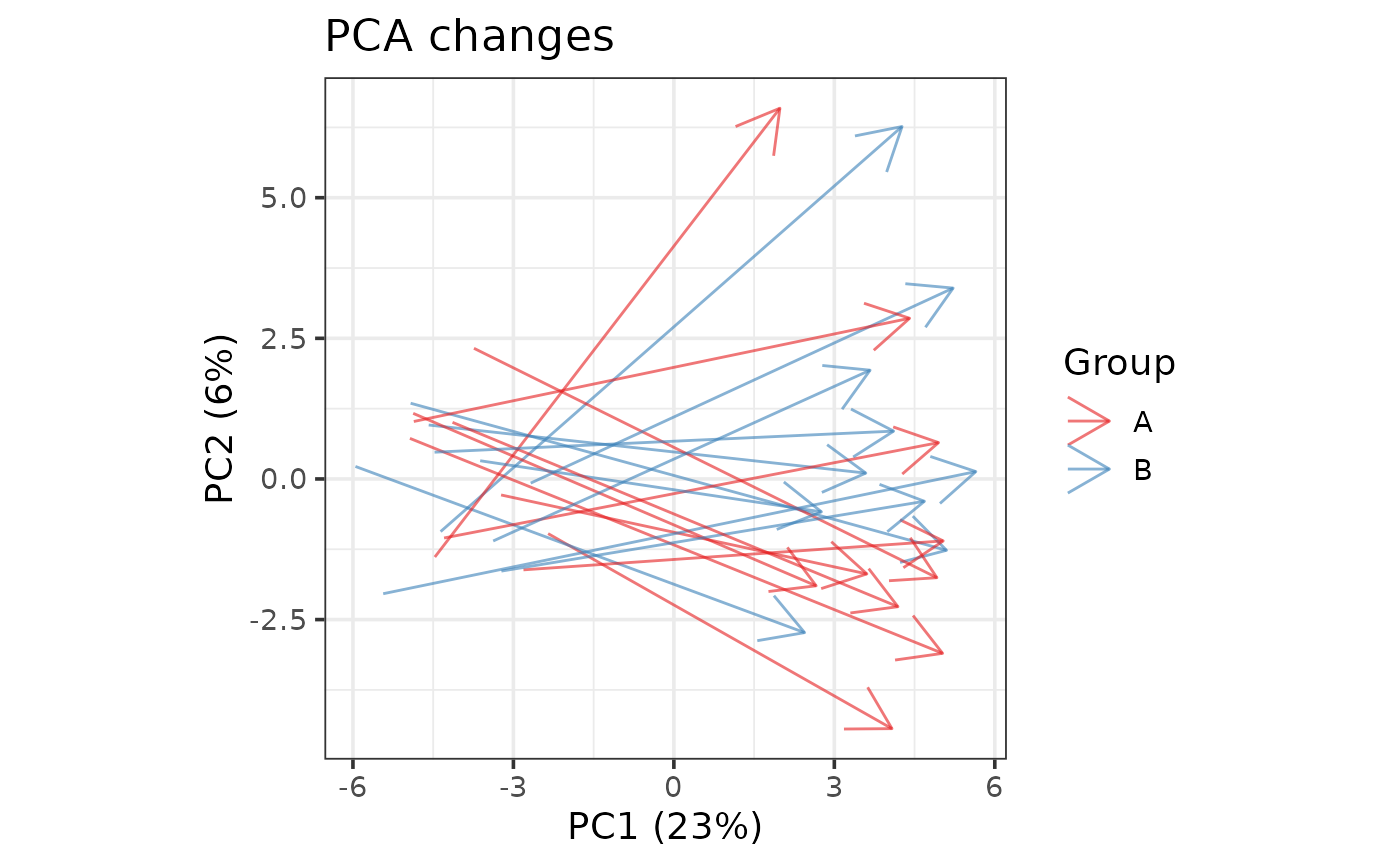
Plots changes in PCA space according to time. All the observations of a single subject are connected by an arrow ending at the last observation.
Usage
plot_pca_arrows(
  object,
  pcs = c(1, 2),
  all_features = FALSE,
  center = TRUE,
  scale = "uv",
  color,
  time,
  subject,
  alpha = 0.6,
  arrow_style = arrow(),
  title = "PCA changes",
  subtitle = NULL,
  color_scale = getOption("notame.color_scale_dis"),
  text_base_size = 14,
  line_width = 0.5,
  assay.type = NULL,
  ...
)
Arguments
- object
a
SummarizedExperimentorMetaboSetobject- pcs
numeric vector of length 2, the principal components to plot
- all_features
logical, should all features be used? If FALSE (the default), flagged features are removed before visualization.
- center
logical, should the data be centered prior to PCA? (usually yes)
- scale
scaling used, as in
prep. Default is "uv" for unit variance- color
character, name of the column used for coloring the arrows
- time
character, name of the column containing timepoints
- subject
character, name of the column containing subject identifiers
- alpha
numeric, value for the alpha parameter of the arrows (transparency)
- arrow_style
a description of arrow heads, the size and angle can be modified, see
?arrow- title, subtitle
the titles of the plot
- color_scale
the color scale as returned by a ggplot function
- text_base_size
the base size of the text
- line_width
the width of the arrows
- assay.type
character, assay to be used in case of multiple assays
- ...
additional arguments passed to
pca
Examples
data(example_set)
plot_pca_arrows(drop_qcs(example_set), color = "Group", time = "Time",
  subject = "Subject_ID")
#> svd calculated PCA
#> Importance of component(s):
#>                  PC1     PC2
#> R2            0.2293 0.06093
#> Cumulative R2 0.2293 0.29024

# If the sample size is large, plot groups separately
plot_pca_arrows(drop_qcs(example_set), color = "Group",
                time = "Time", subject = "Subject_ID") +
  facet_wrap(~Group)
#> svd calculated PCA
#> Importance of component(s):
#>                  PC1     PC2
#> R2            0.2293 0.06093
#> Cumulative R2 0.2293 0.29024
# If the sample size is large, plot groups separately
plot_pca_arrows(drop_qcs(example_set), color = "Group",
time = "Time", subject = "Subject_ID") +
facet_wrap(~Group)
#> svd calculated PCA
#> Importance of component(s):
#> PC1 PC2
#> R2 0.2293 0.06093
#> Cumulative R2 0.2293 0.29024